Introduction

Neural networks (NNs) are all the rage right now and can seem kind of magical at times. In reality, most NNs are essentially just a bunch of logistic regressions¹ stacked on top of each other + a clever way of distributing blame for the predictions and updating the weights accordingly. In this handout, we will break NNs down step-by-step to hopefully de-mystify. There are exercises along the way, but I suggest reading through the whole document before doing them to have a better understanding of the big picture.

I have tried to minimize the math and keep linear algebra out of the way. Implementations of neural networks in libraries such as torch, keras/tensorflow etc. use matrix multiplications and other linear algebra instead of what I’ll show you here². The reason for doing it this way, is that it, at least for me, is far more intuitive to see what happens at each individual node. Once you understand this, understanding how it’s done with linear algebra is not as daunting.

Let’s begin our journey by understanding activation functions.

Activation functions

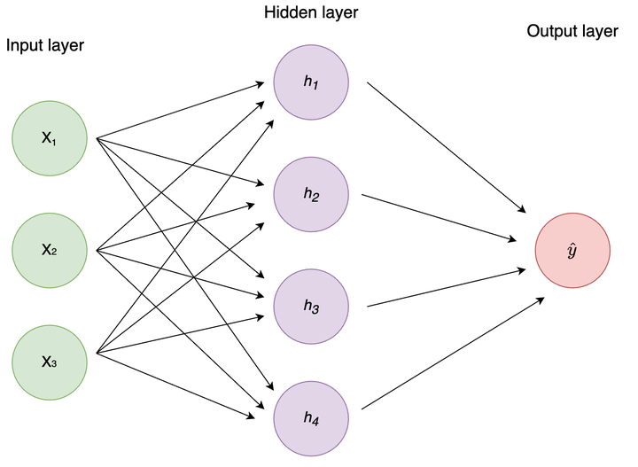
Consider a standard feedforward neural network (aka multilayer perceptron)

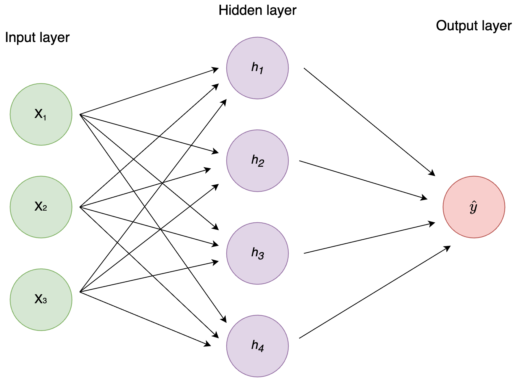
Figure 1: Figure 1: Standard MLP

This network takes 3 inputs (a row of 3 variables/columns in your data), has 4 hidden nodes, and a single output node which means it will output a single number. For regression and binary classification you use a single output node, and for multiclass classification you use an output node per group.

Upon creation of the network, all weights between the nodes (i.e. the links/lines in the image) are initiated with a random value³. When the networks get an input of training examples, the inputs are multiplied by the weights and fed to the next layer of nodes. In our case, each node in the hidden layer receives an input which is a vector of 3 elements: the input times the weight from each input node to the hidden node. Before the hidden node can propagate the signal forward, it has to aggregate it to a single number with a non-linear function.⁴ This is where the activation function comes in.

Nowadays, ReLU (and its variants) is the most common activation function, but sigmoid is the OG. The equations are as follows:

\[ReLU = max(0, input)\] \[sigmoid = \frac{1}{1+e^{-input}}\] The input in the above equations refers to the net input to the nodes, i.e. the weighted sum of all inputs. All the activation function does, is apply some function to the net input. This becomes the node’s activation and is what is fed to the next layer of nodes in the network in exactly the same manner as from the input to the first hidden layer.

Let’s see a quick example of how to calculate activation for a single hidden node with 3 input nodes. Let’s assume this is the top hidden node in Figure 1, \(h_1\).

# Assume we get an input of (1, 3, 5) in
# x1, x2, x3 respectively
input_nodes <-  c(1, 3, 5)

# these are weights coming into h1
# first element from x1, second from x2 etc
weights_i_h1 <-  c(0.5, 1.2, -0.3)

(weighted_input <-  input_nodes * weights_i_h1)

## [1]  0.5  3.6 -1.5

(net_input <- sum(weighted_input))

## [1] 2.6

# Define our activation functions 
sigmoid <- function(x) 1 / (1+ exp(-x))
relu <- function(x) max(0, x)

# Calculate activations
# Note: each node only has 1 activation function. 
# I showed both here to illustrate the difference between them
(h1_activation <- sigmoid(net_input))

## [1] 0.9308616

relu(net_input)

## [1] 2.6

Visually, this is what’s happening.

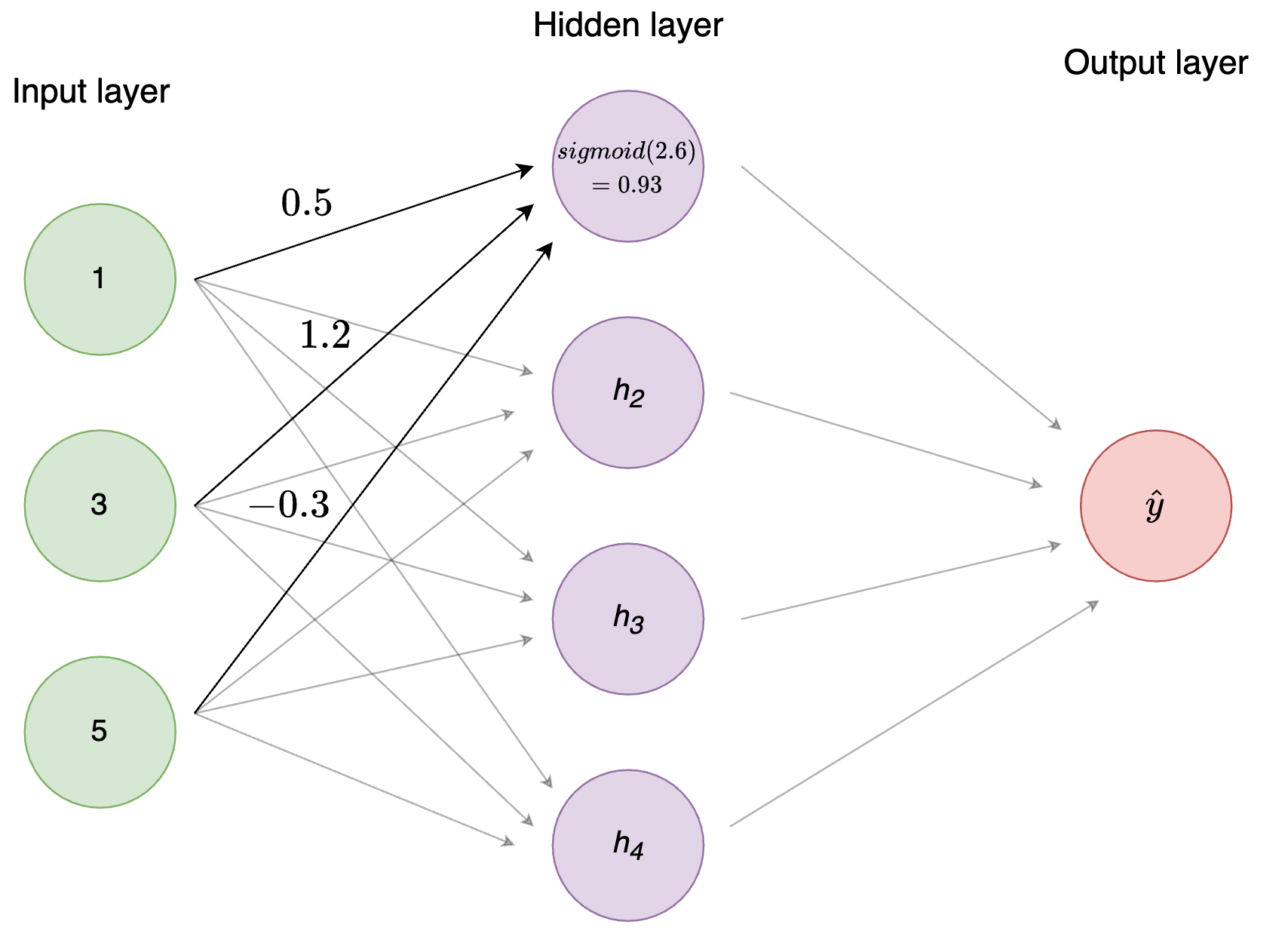
Figure 2: Figure 2: Activation function

Repeat the process for all the nodes in the network and voíla - you just implemented the forward pass of a neural network!⁵

Notice how similar this is to logistic regression: You have a bunch of input nodes/variables, which have an associated weight (betas), which are combined using the sigmoid (aka logistic) function.

Note: each node also has a bias which is an extra trainable parameter (essentially an intercept). For simplicity we assume it to be zero here.

Gradient descent

Hurray, the forward pass is done! The network is just making random predictions for now though, so we need to give it a way to learn. This is where backpropagation and gradient descent comes in. Now, as with any regression model, we need to define some loss function, i.e. how we calculate the “goodness” of the model. The loss function to use depends on the problem at hand, but a common one for regression is sum of squares errors. The equation is very straightforward and looks like this:

\[SSE = \sum^n_{i=1}(y-\hat{y})^2\] Where \(y\) is the label and \(\hat{y}\) your prediction. The greater the distance your prediction is from the target, the larger the SSE is. Therefore, we want to minimize this.

From high school calculus, you might recall that the derivative of a function is simply the slope of the function. ⁶

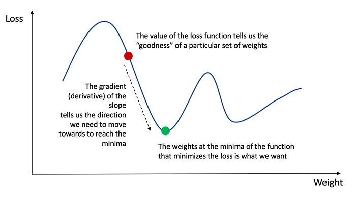
(#fig:grad_desc)Figure 3: Loss landscape

The plot above is an illustration of the loss (e.g. the SSE) given different combinations of weights between nodes.⁷ As the image illustrates, if we are unlucky we can get stuck in local minima, i.e. an area where the gradient is zero, but that is not the global minimum, i.e. the combination of weights with the lowest possible loss. This is just a fact of life for neural networks - you are in no way guaranteed to find the optimal solution. Different weight initializations will lead you to find different minima, which can vary substantially.

Anyhow, the way we minimize the loss is to calculate the gradient of the loss function in our current state and make changes to our weights based on this. The sign (+ or -) of the gradient tells us which direction to go, and the magnitude tells us how large steps to take. In essence, we start at some random point on the graph above, and slowly make our way down, until we hopefully end at the green dot.

The procedure differs slightly if the node is an output or hidden node. Let’s go through it for output nodes first.

In our case, we had a single output node, so let’s assume we’re doing binary classification (is it a 0 or a 1?).⁸ For binary classification, it makes sense to use the sigmoid as activation function for our output, as it squishes the values to a range between 0 and 1. To calculate the derivative of the loss function with respect to the weights (and biases), \(\delta\), we need to use the chain rule which eventually gives us this⁹:

\[ \begin{aligned} \delta &= \textrm{the derivative of the loss function} \cdot \\& \textrm{the derivative of the activation function} \end{aligned} \]

Using SSE and sigmoid activation function we get this:

\[\delta = 2(y-\hat{y}) \cdot a(1-a)\]

Where \(a\) is the node’s activation, i.e. the value we get after using the activation function (sigmoid) on the sum of the weighted input.

Let’s see an example calculation.

# assume the true label of the target is 1
label <-  1

# assume that the activation of the output
# node (after the entire forward pass) is 0.6
output_node_activation <- 0.6

# Derivative of the sigmoid function:
sigmoid_derivative <- function(x) x*(1-x)

(delta_o <- 2*(label - output_node_activation) * 
    sigmoid_derivative(output_node_activation))

## [1] 0.192

Visually, this is what’s happening.

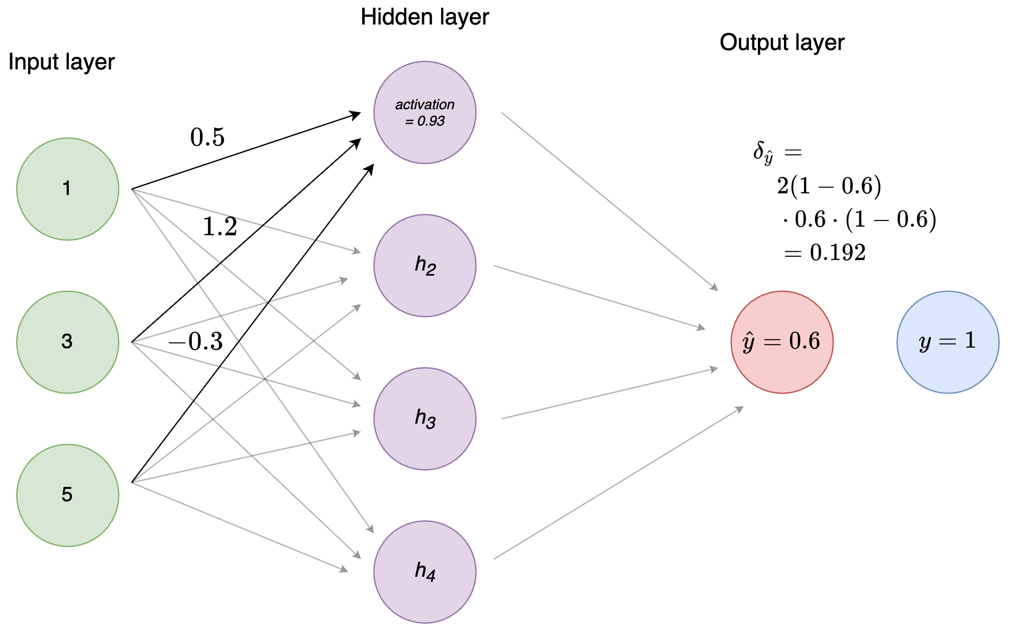
Figure 3: Figure 4: Calculation of \(\delta\) of the output node

Easy! Notice that the value of \(\delta\) is positive. This is because our prediction (0.6) was below the label (1) and we should therefore increase the weights to get closer to the correct prediction. Had the label been 0 instead, \(\delta\) would have been a negative number. Essentially, \(\delta\) tells us how we should make changes to our weights to get closer to the optimal state as defined by the loss function.¹⁰

The clever thing about backpropagation is that weights are updated based on their magnitude. That is, if the error is large, large activations will change more than small activations, as they “contribute” more to the prediction than the smaller ones. As the name implies, the errors are propagated back into the network (what is known as the backward pass). Calculating \(\delta\) for the hidden layer is the first step in this process.

Now, to distribute blame for the prediction.

Backpropagation

As mentioned, backpropagation works a bit differently whether you’re calculating weights coming in to an output or a hidden node. For weights coming in to the output nodes, the weight changes are proportional to the learning rate \(\eta\), the activation of the predecessor node, and the \(\delta\) we just calculated. To continue with our example from Figure 1, let’s calculate the weight changes for the weight going from the top hidden node \(h_1\) to the output \(\hat{y}_1\).¹¹

# Assume a random weight
# from h1 to yhat (calling yhat 'o' for output)
weight_h1_o <- c(0.8)


# To calculate the weight change we need:
# 1) the activation of the input unit
#   which in this case is h1
# 2) the delta of the output unit
# 3) a learning rate (alpha)

# Learning rates differ a lot
# but let's go with 0.01
alpha <- 0.01

# plugging numbers into the equation
(weight_change <- alpha * delta_o * h1_activation) 

## [1] 0.001787254

# update weight
(weight_h1_o <- weight_h1_o + weight_change)

## [1] 0.8017873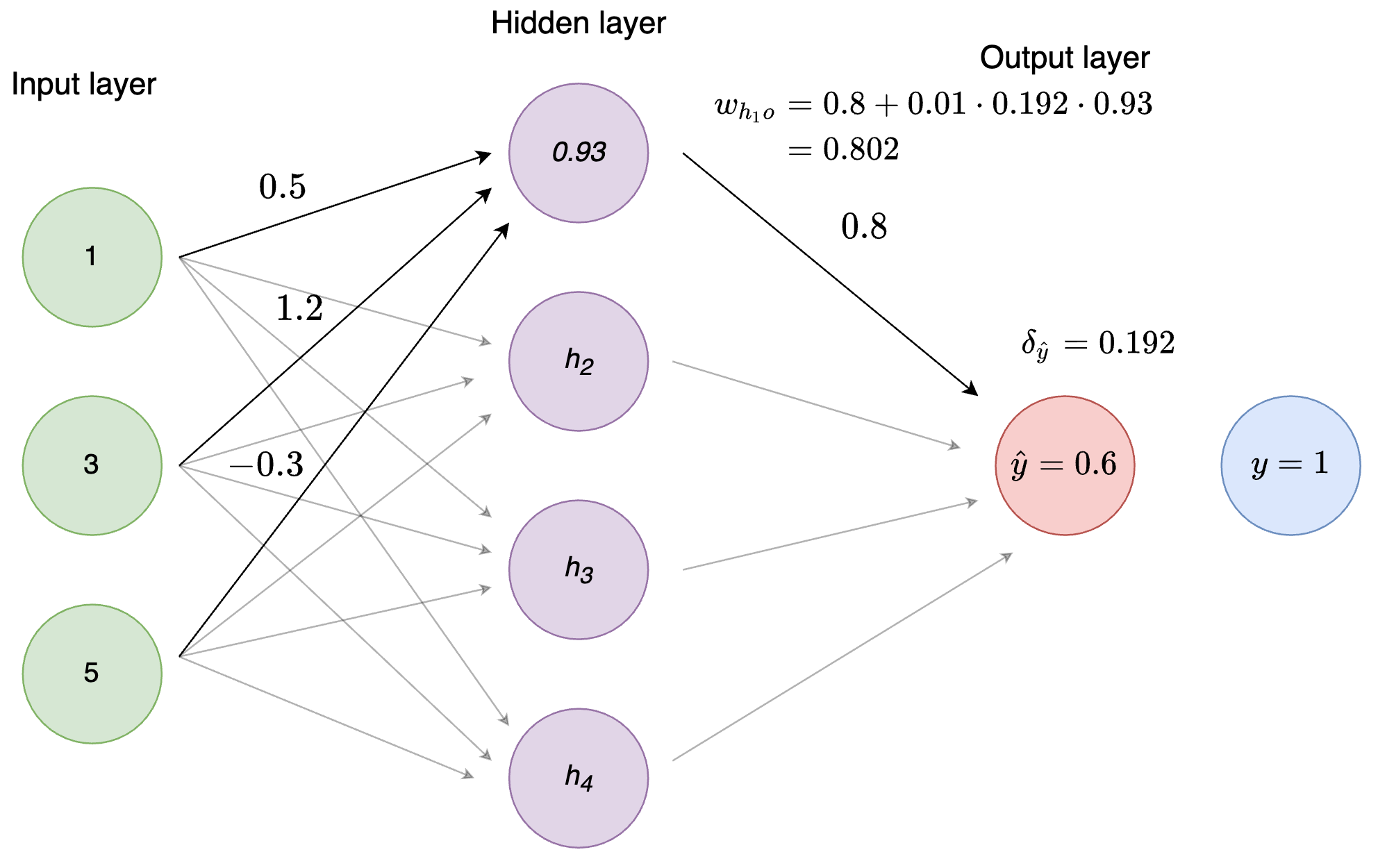

Figure 4: Figure 5: Weight updating

Pretty easy right? To calculate the weight change for weights going into hidden units, we simply multiply the learning rate, \(\alpha\) with the \(\delta\) (the derivative of the loss function with respect to the weights) and the activation at the preceeding node.

\[\text{weight change} = \alpha \cdot \delta \cdot activation\]

We’re getting really close to having trained our little NN on a single example. All that’s left is calculating the weight changes for the weights from the input nodes to the hidden nodes. Fortunately, the procedure is largely the same as for the output units.

First, we calculate \(\delta\) for the specific weight and node again. However, since we are now in the hidden layer, we don’t have access to the true label anymore. Instead, we use the \(\delta\) from the succeeding layer (the output node) multiplied by the weight from our hidden node to the output!

To calculate \(\delta\) for the hidden node, \(\delta_{h_1}\), we sum over all the \(\delta \cdot weight\) for the output node and multiply by the derivative of the activation. In other words, we calculate delta_o_times_weight_h1 + delta_o_times_weight_h2 + delta_o_times_weight_h3 + delta_o_times_weight_h4 and multiply by the derivative of the activation of \(h_1\). Let’s see an example.

# Using the weight we calculated before
# and setting 3 random weights for h2_o, h3_o, h4_o
weights_h_o <- c(weight_h1_o, 0.5, 0.1, 0.6)

(delta_o_times_weights <- delta_o * weights_h_o)

## [1] 0.1539432 0.0960000 0.0192000 0.1152000

(sum_delta_o_times_weights <- sum(delta_o_times_weights))

## [1] 0.3843432

(delta_h1 <- sum_delta_o_times_weights * 
  sigmoid_derivative(h1_activation))

## [1] 0.02473567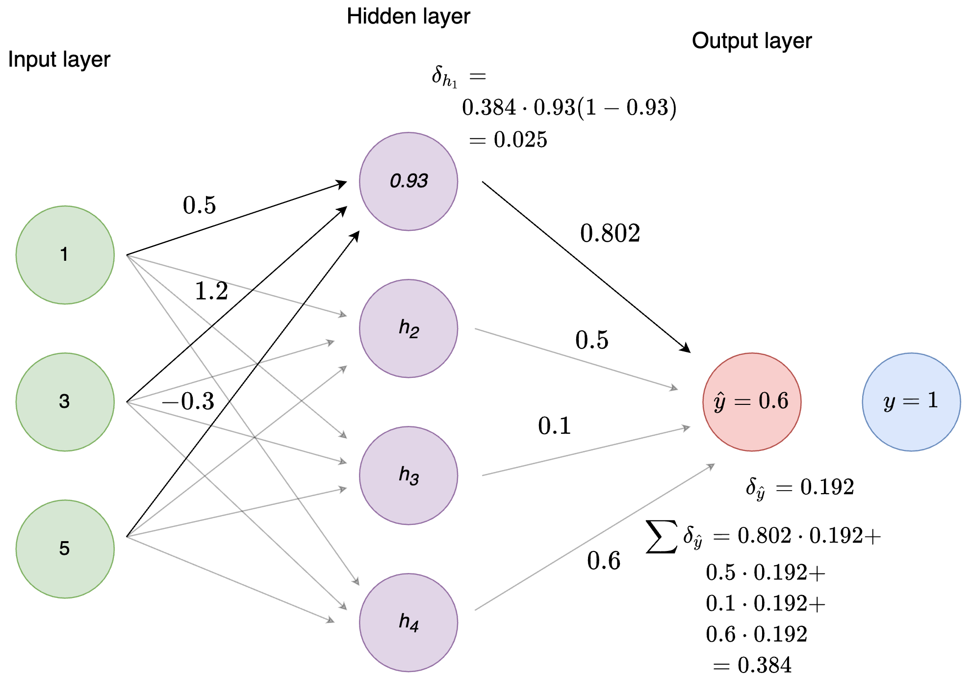

Figure 5: Figure 6: Calculation of \(\delta_{h_1}\)

Notice that the value of \(\delta\) is substantially smaller than what it was at the output nodes. This means that the weight changes from the input nodes to the hidden nodes will be even smaller. Deep networks can run into the problem of vanishing gradients, i.e. \(\delta\) becomes so small that weight changes are negligible. ReLU is far more robust to the problem of vanishing gradients than the sigmoid function, which is one of the reasons for its success.

Alright, we’re getting reeally close now. The last step to update the weights coming in to the hidden nodes is exactly the same as for the weights coming in to the output node: \(\alpha \cdot \delta \cdot activation\)

We already defined our 3 input nodes and their weights going to \(h_1\). Let’s update them.

(weight_change <- alpha * delta_h1 * input_nodes)

## [1] 0.0002473567 0.0007420701 0.0012367836

(weights_i_h1 <- weights_i_h1 + weight_change)

## [1]  0.5002474  1.2007421 -0.2987632

And we’re done! Rinse and repeat for the rest of the hidden nodes and you just trained one step of a neural network! For a standard feedforward neural network, this is all that is going on - just repeated a lot of times.¹² When this process has been conducted for each training example, the neural network has gone through one epoch. You usually stop training after a certain number of epochs, or once you reach a stopping criterion.¹³

Doesn’t seem so magical anymore, right?

To sum up, here are the steps:

1. Initialize the network: Randomly initialize all the weights.

2. Forward pass: Pass an input to the neural network and propagate the values forward. To calculate activation of the nodes, take the weighted sum of their input and use an activation function such as the sigmoid or ReLU.

3. Backward pass: Calculate the loss for your current training example. Calculate \(\delta\) for the output node(s) and update the weights coming in to the output node(s) by multiplying \(\delta\) with the learning rate and the activation of the hidden node feeding into the output node. Continue this process by propagating \(\delta\) back into the hidden layers and continually updating the weights.

4. Repeat: Repeat for a specific number of epochs or until some stopping criterion is reached.

References and further reading